Consider Again the Discrete Time Feedback System of Example

1. Introduction

The design of command systems for multivariable plants is a wide research topic that is still subject to considerable worldwide interest. Systems with multiple input and output variables often deliver challenges and opportunities that are not available in the Single-Input Single-Output (SISO) plants. For case, in the Multi-Input Multi-Output (MIMO) approach, the Inverse Model Control (IMC) extends the potential of nonunique solutions for a given trouble [1,2,three,4,5,half-dozen,7].

One of the most popular inverse model controls is the Minimum Variance Control (MVC) used for both discrete and continuous plants [eight,ix,ten,11]. On the other hand, the perfect control, beingness a deterministic equivalent of MVC, has been developed mainly for the discrete-time framework. Therefore, some efforts to ascertain the Continuous-Time Perfect Command (CTPC) have recently been undertaken [12]. The preliminary studies have shown that this topic is yet an unexplored expanse of control theory. Thus, a new approach to CTPC design is confirmed within this paper.

The key part of perfect control synthesis for multivariable systems is the proper solution of inverse problem derived from the control police force. For decades, the unique Moore–Penrose changed has been used due to its minimum-norm holding [xiii,14,xv,16,17,18]. On the other hand, admission of the nonunique inverses has resulted in measurable benefits in terms of control speed, energy minimization, or control stability [xix]. Thus, in this paper, a short comparing of 2 selected inverses, namely, unique (Moore–Penrose) right T-inverse and nonunique right

$\sigma$

-inverse, is shown. Of form, this comparison will exist conducted in the context of CTPC employment.

Stability of such a control scenario volition exist analyzed with the awarding of well-known land-feedback or pole-placement methods [20,21]. Additionally, in contrast to the preliminary studies [12], here, the state-feedback form is given in a straightforward style, allowing us to obtain the closed-loop poles immediately for all classes of LTI MIMO state-infinite systems [22]. Of course, equally in the detached-time equivalent, the stability should be understood in terms of the Bounded-Input Divisional-State (BIBS) or input-to-state approach [23].

However, both control law analysis and synthesis will exist made using continuous-time solvers provided by some incremental time-originated stride

$\Delta t$

, which can be found, e.k., in the Matlab surround [24,25]. The influence of the time interval volition exist taken into account during the entirety of the process of perfect control realization and validation.

This paper is organized equally follows. After a short introduction, the system clarification is given. In Department 3, a brief reminder considering unique and nonunique inverses of nonsquare matrices is presented. The crucial CTPC law is given in Section 4, together with the full calculation procedure covering its closed-loop behavior. Discussion over stability of such a perfect control constitute is made with respect to the solver-related peculiarities, leading to interesting observations shown in Section five. Simulation written report given in the penultimate department shows that the proposed control law tin successfully be applied in the Matlab/Simulink environs. Finally, the conclusions and open problems are manifested.

2. Organization Representation

As the perfect command algorithm reveals its characteristics for multivariable plants, the organization is considered hither as an LTI country-space establish described in the continuous-time domain as follows:

$$\left\{\begin{array}{cc}\dot{\mathbf{x}}\left(t\right)=\mathbf{A}\mathbf{x}\left(t\right)+\mathbf{B}\mathbf{u}\left(t\right),\hfill & \mathbf{x}\left(0\right)={\mathbf{x}}_{\mathbf{0}}\hfill \\ \mathbf{y}\left(t\right)=\mathbf{C}\mathbf{x}\left(t\right)\hfill \end{array}\right.,$$

(ane)

where

$\mathbf{A}\in {\mathbb{R}}^{n\times \mathrm{due\; north}}$

,

$\mathbf{B}\in {\mathbb{R}}^{n\times {\mathrm{north}}_u}$

and

$\mathbf{C}\in {\mathbb{R}}^{{\mathrm{due\; north}}_y\times \mathrm{north}}$

are organization input and output matrices, respectively. Moreover

$\mathbf{u}\left(t\right)$

,

$\mathbf{y}\left(t\right)$

, and

$\mathbf{x}\left(t\right)$

are

$n_u$

-input,

$n_y$

-output, and n-land vectors, respectively. Every bit in all state-space-based scenarios, nosotros additionally define the state initial condition

${\mathbf{x}}_{\mathbf{0}}$

vector equivalent to the

$\mathbf{10}\left(t\right)$

for

$t=0$

.

Remark1.

Due to the nature of the perfect control police, we rather chose to omit the systems with $n_u<{\mathrm{due\; north}}_y$. For such plants, it is shown—eastward.g., in Ref. [26]—that the perfect command cannot be established.

Earlier we continue of the perfect command algorithm, permit us remember the concept concerning nonunique matrix inverses. These inverses volition afterwards be used in order to establish the perfect command police; thus, inverse-oriented preliminaries are given in the adjacent section.

3. (Non)unique Right Inverses

The idea of nonsquare matrix right inverses is built upon the statement of finding such a matrix

${\mathbf{M}}^{\mathrm{R}}$

that for a given matrix

$\mathbf{M}$

, the following relation

holds. For nonsquare matrices, this can be accomplished using several frameworks, resulting in both unique and nonunique solutions [27,28]. The most popular is the unique minimum-norm Moore–Penrose T-inverse as follows:

$${\mathbf{M}}_0^{\mathrm{R}}={\mathbf{M}}^{\mathrm{T}}{\left(\mathbf{M}{\mathbf{M}}^{\mathrm{T}}\right)}^{-1},$$

(iii)

where the full-rank matrix

$\mathbf{Yard}$

needs to have more columns than rows to achieve the holding chosen right-invertibility. On the other hand, there is also a broad range of nonunique inverses available during the perfect control design. For case, the right

$\sigma$

-changed can be given in the following course [29]

$${\mathbf{K}}_{\sigma }^{\mathrm{R}}={\beta }^{\mathrm{T}}{\left(\mathbf{Thousand}{\beta }^{\mathrm{T}}\right)}^{-1},$$

(iv)

where

$\beta$

—being of the same sizes as

$\mathbf{M}$

—provides a ready of the so-called degrees of liberty. Of course, the additional limitation is only that the matrix

$\left(\mathbf{1000}{\beta }^{\mathrm{T}}\right)$

is expected to exist a full rank. The application of correct

$\sigma$

-changed has already proven its usefulness during the perfect command design. For instance, in Refs. [19,28,30], it was shown that the proper caste-of-freedom selection enables to obtain, due east.g., pole-free, robust, or minimum-free energy perfect command beliefs. Even so, the said advantages were obtained for discrete-time plants only; thus, permit united states of america now keep with the perfect control algorithm for continuous-time systems. Therefore, this control strategy, divers in terms of the state-feedback organization, is proposed in the next section. Detect that the discussed new arroyo is strictly dedicated to any MIMO plant with

${\mathrm{north}}_u⩾n_y$

. The predecessor provided by Ref. [12] has only employed the systems with right-invertible country-infinite-related matrices

$\mathbf{B}$

. The boosted improvement, in comparison to the algorithm given in Ref. [12], is the fact that there is no longer a need to switch between two operating-time-originated ranges.

4. New Perfect Command Law

The perfect control algorithm has already been developed for discrete-time systems. The main property obtained for such procedure is minimum possible control error that vanquishes immediately later a single simulation pace (for plants with unit state delay). In this particular piece of work, we are targeting similar found beliefs, just for systems described in the continuous-time state-space framework. In both cases, the main concern is to minimize a performance index, which, for the continuous-time scenario, tin be described as follows:

$$J=\left|\right|{\mathbf{y}}_{\mathbf{ref}}\left(t\right)-\mathbf{y}\left(t\right){\left|\right|}_{\mathrm{ii}},$$

(5)

where symbols

${\mathbf{y}}_{\mathbf{ref}}\left(t\right)$

and

$\mathbf{y}\left(t\right)$

denote the reference value/setpoint and output of a system, respectively. Having such an index, we tin can attempt to obtain a like minimum-error property as resulted in the discrete-time approach [31]. The study presented here is based on the important derivative of vector

$$\dot{\mathbf{y}}\left(t\right)=\mathbf{C}\dot{\mathbf{x}}\left(t\right),$$

(6)

allowing us to determine the operation of output variable. Now, aiming for the perfect control strategy with maximum accurateness (in terms of assumed norm (5)), we can introduce an equation minimizing the control error in the following manner

$$\dot{\mathbf{y}}\left(t\right)={\mathbf{y}}_{\mathbf{ref}}(t+\Delta t)-\mathbf{y}\left(t\right).$$

(7)

Of course, in such a scenario, the current control error is driven to zero immediately. However, at this moment, we need to acknowledge the fact, that solvers implemented in the Matlab environment are in fact based on nonzero fixed or adaptive footstep time

$\Delta t$

; thus, nosotros tin unarguably write the subsequent formula

$$\dot{\mathbf{y}}\left(t\right)=\frac{d\mathbf{y}\left(t\right)}{dt}\approx \frac{\mathbf{y}(t+\Delta t)-\mathbf{y}\left(t\right)}{\Delta t}.$$

(viii)

Naturally, this supposition is valid under

$\Delta t\to 0$

. Information technology is clear at present that the main aim here is to obtain system output behavior described by the following relation

$$\dot{\mathbf{y}}\left(t\right)=\frac{{\mathbf{y}}_{\mathbf{ref}}(t+\Delta t)-\mathbf{y}\left(t\right)}{\Delta t},$$

(9)

then the output fault shall disappear right after the step time that is inherent to solver parameters. Again, information technology is needed to emphasize that guaranteeing the output derivative equal to the electric current control error will minimize the operation index given in Equation (5). Now, using the output description from Equation (i), one can write the post-obit outcome

$$\mathbf{C}\dot{\mathbf{x}}\left(t\right)=\frac{{\mathbf{y}}_{\mathbf{ref}}(t+\Delta t)-\mathbf{C}\mathbf{x}\left(t\right)}{\Delta t},$$

(10)

where all parameters are known for systems with given initial weather. Based on the above, i tin can obtain the perfect command formula by the proper mathematical manipulations

$$\mathbf{C}(\mathbf{A}\mathbf{10}\left(t\right)+\mathbf{B}\mathbf{u}\left(t\right))\Delta t={\mathbf{y}}_{\mathbf{ref}}(t+\Delta t)-\mathbf{C}\mathbf{x}\left(t\right).$$

(eleven)

At present, the event is to extract the control signal

$\mathbf{u}\left(t\right)$

from the above presented expression. This involves the crucial matrix inverse providing an infinite number of possible solutions for the discussed complex problem. Finally, let usa introduce the perfect command police force for continuous-fourth dimension LTI MIMO state-infinite systems in the grade of

$$\mathbf{u}\left(t\right)=-{\left(\mathbf{CB}\right)}^{\mathrm{R}}\mathbf{C}(\mathbf{A}+\mathbf{I}\frac{\mathrm{one}}{\Delta t})\mathbf{x}\left(t\right)+{\left(\mathbf{CB}\right)}^{\mathrm{R}}\frac{1}{\Delta t}{\mathbf{y}}_{\mathbf{ref}}(t+\Delta t),$$

(12)

where superscript '

$\mathrm{R}$

' denotes any right inverse, particularly the right

$\sigma$

- and T-inverse covered in Department 3. Of course, for a zero reference value, the perfect command formula reduces to the perfect regulation every bit follows:

$$\mathbf{u}\left(t\right)=-{\left(\mathbf{C}\mathbf{B}\right)}^{\mathrm{R}}\mathbf{C}(\mathbf{A}+\mathbf{I}\frac{1}{\Delta t})\mathbf{10}\left(t\right).$$

(13)

Note that the dynamics of a institute can similarly be examined for both zero- and nonzero-referenced setpoints.

Remark2.

Interestingly, the detached-time perfect control scenario implies the input formula divers past

$$\mathbf{u}\left(k\right)=-{\left(\mathbf{CB}\right)}^R\mathbf{CAx}\left(\mathrm{grand}\right).$$

(14)

The just obtained similarity is remarkable; notwithstanding, the continuous-time perfect control police force converges only for $\Delta t\to \infty$.

Referring to the conducted investigations, the formal determination is given below.

Theorem1.

Let united states consider the LTI MIMO systems (1) with $n_u⩾{\mathrm{due\; north}}_y$ described in the continuous-time state-space framework. The continuous-fourth dimension perfect control police for such a class of plants is divers every bit follows:

$$\mathbf{u}\left(t\right)=-{\left(\mathbf{CB}\right)}^{\mathrm{R}}\mathbf{C}(\mathbf{A}+\mathbf{I}\frac{1}{\Delta t})\mathbf{x}\left(t\right)+{\left(\mathbf{CB}\right)}^{\mathrm{R}}\frac{\mathrm{ane}}{\Delta t}{\mathbf{y}}_{\mathbf{ref}}(t+\Delta t),$$

(fifteen)

under an arbitrary initial condition ${\mathbf{ten}}_{\mathbf{0}}$.

Proof.

Immediately after combining the system's description (ane) with expression (xv), we receive

$$\dot{\mathbf{y}}\left(t\right)=-\mathbf{C}\frac{\mathrm{ane}}{\Delta t}\mathbf{x}\left(t\right)+\frac{1}{\Delta t}{\mathbf{y}}_{\mathbf{ref}}(t+\Delta t),$$

(xvi)

which holds the examined perfect-command-oriented target in the form of

$$\dot{\mathbf{y}}\left(t\right)=\frac{{\mathbf{y}}_{\mathbf{ref}}(t+\Delta t)-\mathbf{y}\left(t\right)}{\Delta t},$$

(17)

provided by

$\Delta t\to 0$

. □

Remarkiii.

Naturally, the condition (17) guarantees a possible minimum perfect control-related error derived from the step time $\Delta t$ tending to cypher. Thus, there is no dependence betwixt the establish inertia and the time-step-size needed to reach the new reference value. Through the sure small $\Delta t$, the corresponding negligible steady-land error is obtained, which ultimately fades in the example of discrete-time perfect control instances.

Remark4.

It seems that operation $\Delta t\to 0$ generates the excessive energy of the perfect control input runs. This intriguing issue should be treated equally an open trouble.

Notice that the controlled output will stay at the reference value in any deterministic case, independently from the dynamics concealed within airtight-loop equations. Thus, the stability of CTPC will be discussed in the next department.

5. Stability Properties of the New Perfect Control Constabulary

The stability of perfect command algorithm has already been discussed widely for a class of discrete-time systems [26]. In the literature, it can be plant that the stability property should be understood in terms of the BIBS approach. It is caused mainly by the fact that the perfect control output remains stable fifty-fifty for plants with closed-loop poles located outside the stable region. Thus, the input-to-state characteristics are the main concern here. Of course, according to Equation (thirteen), the CTPC algorithm can be treated as the inverse model control-oriented state-feedback system occupied by

$$\mathbf{u}\left(t\right)=-\mathbf{Kx}\left(t\right),$$

(xviii)

where

$\mathbf{Chiliad}={\left(\mathbf{CB}\right)}^R\mathbf{C}(\mathbf{A}+\mathbf{I}\frac{1}{\Delta t})$

, whose closed-loop control poles tin can exist calculated in accordance with the following formula

$$d\mathrm{eastward}t(\mathbf{A}-\mathbf{B}\mathbf{K})=0.$$

(19)

It is clear that the discussed stability depends on the part connecting vectors

$\mathbf{x}\left(t\right)$

and

$\dot{\mathbf{10}}\left(t\right)$

; thus, the airtight-loop poles tin be obtained. The static not-autoregressive part disappears as soon every bit the output reaches its reference value, which substantially occurs after a single calculation step

$\Delta t$

. In conclusion, the stability of the closed-loop CTPC law is adamant past the roots of characteristic equation as follows:

$$d\mathrm{due\; east}t(s\mathbf{I}-\mathbf{A}+\mathbf{B}{\left(\mathbf{C}\mathbf{B}\right)}^{\mathrm{R}}\mathbf{C}(\mathbf{A}+\mathbf{I}\frac{1}{\Delta t}))=0.$$

(20)

Here again, we need to emphasize that the numerical solution of stability problem can exist considered in the context of the inverse matrix adding, with an space number of possible outcomes—even with the ability to almost capricious allocation of the number of zero and nonzero airtight-loop poles.

Remarkv.

The pole-placement characteristic is connected with the rank of the closed-loop perfect control system matrix. The mentioned rank seems to exist dependent on the size differences derived from $\mathbf{A}$,$\mathbf{B}$,$\mathbf{C}$ matrices. This intriguing phenomenon is nevertheless under investigation.

Interestingly, in comparison with the detached-time instances, the zero closed-loop poles are not obtained here. This is caused past the fact that the additional role of country feedback

$\left(\mathbf{I}\frac{1}{\Delta t}\right)$

entails a drift of the CTPC algorithm poles that were originally equal to zero. In this example, the zero eigenvalues of the closed-loop system matrix are transformed to those connected with the solver-derived

$\Delta t$

parameter. The influence of solver time seems to be an obvious consideration when aiming for proper output beliefs. If the goal is to obtain the zero control error in a single solver step, it is clear that if the solver step takes a shorter fourth dimension

$\Delta t$

, and then the dynamics applied to the output and state variables should be faster to overcome the shorter calculation interval.

In order to explain the crucial office of the step time

$\Delta t$

, the closing statements are formulated beneath.

Theorem2.

The continuous-time perfect command law as in Equation (12) should be understood in terms of the single stride time $\Delta t$ tending to cypher.

Proof.

Immediately afterward commutation of Formula (12) to correct-invertible nondelayed plants (one), we obtain the expression

$$\dot{\mathbf{y}}\left(t\right)=\frac{1}{\Delta t}\left({\mathbf{y}}_{\mathbf{ref}}(t+\Delta t)-\mathbf{y}\left(t\right)\right),$$

(21)

which can be transformed, according to the relation (vii), to

$$\left(\frac{\Delta t-1}{\Delta t}\right)\left[{\mathbf{y}}_{\mathbf{ref}}(t+\Delta t)-\mathbf{y}\left(t\right)\right]=\mathbf{0}.$$

(22)

For

$\Delta t\to 0$

, we receive

$\mathbf{y}\left(t\right)\to {\mathbf{y}}_{\mathbf{ref}}(t+\Delta t)$

, which ends the proof. □

Corollaryone.

The perfect regulation (13) having ${\mathbf{y}}_{\mathbf{ref}}\left(t\right)=\mathbf{0}$ occurs iff the relation

$$\Delta t\mathbf{y}\left(t\right)=\mathbf{y}\left(t\right),$$

(23)

determined by $\Delta t\to 0$, $\mathbf{y}\left(t\right)\to 0$, holds.

Remark6.

The stability of the CTPC should be considered in the same manner.

Remarkvii.

It would be interesting to extend the new theory to the case of plants involving the fourth dimension-delay-originated $\Gamma \left(s\right)={\mathrm{eastward}}^{-s{T}_0}$ term defined in the Laplace domain.

Having divers all crucial properties of CTPC systems, let united states of america now go on with a simulation study. The proposed control schemes will be tested together with predicted closed-loop poles beliefs. Instances made using the Matlab/Simulink environment are presented in the side by side department.

six. Simulation Examples

It has been shown in previous studies apropos the perfect command simulation for discrete systems that the awarding of nonunique right inverses is useful in the stabilization of nonminimum-phase plants [32]. In this section, we expect to notice similar properties for continuous-time objects. Moreover, there is a need to assess the system stability, especially in the context of the closed-loop poles presence. Thus, three different instances volition be considered in this section in club to examine all analyzed behaviors. At this point, it is crucial to emphasize that the Matlab/Simulink surround was used in this study. Moreover, the sampling fourth dimension of the

$ode1$

solver was set to

$\Delta t$

for a reasonable information drove.

6.i. Two-By-One System

In the first simulation scenario, nosotros consider the continuous-fourth dimension LTI system with two inputs, i output, and two state variables described in the state-space framework that is under the post-obit matrices

$\mathbf{A}=\left[\begin{array}{cc}-0.21& -\mathrm{0.twoscore}\\ 0.20& -0.37\end{array}\right]$

,

$\mathbf{B}=\left[\begin{array}{cc}\mathrm{i.10}& -0.70\\ 0.50& -1.00\end{array}\right],$$\mathbf{C}=\left[\begin{array}{cc}-0.90& -\mathrm{0.forty}\end{array}\right]$

and initial status

${\mathbf{x}}_0^{\mathrm{T}}=[3-\mathrm{v}]$

. Additionally, we declare that the simulation step time is equal to

$\Delta t=0.1$

s. Every bit we can see, this plant is stable, since the open up-loop eigenvalues are equal to

$s_{\mathrm{ane},\mathrm{ii}}=-0.2900\pm 0.2713i$

. For such a organization, let united states of america design the perfect control scheme guaranteeing the law from (12). In this scenario, we use the minimum-norm correct T-inverse of (3).

Equally nosotros can detect, a steady-land zip-mistake output is obtained here just after a single calculation step (see Figure ane). Once more, the calculation stride

$\Delta t$

shall exist recalled again, as it affects the possible solution of stability criteria mentioned in the previous section. Thus, we obtain the closed-loop perfect control arrangement matrix

$$\mathbf{A}-\mathbf{BK}=\left[\begin{array}{cc}-7.4965& -3.2618\\ -5.6328& -2.6609\end{array}\right],$$

(24)

and, according to Equation (twenty), our poles are equal to

$s_1=-\mathrm{x.0000}$

and

$s_2=-0.1574$

. Of course, with such a solution, this system is stable.

The resulted stable state and control signals tin can exist observed in Figure one.

Remarkeight.

Alternatively, with the use of the classical airtight-loop poles definition from (19), the eigenvalues $s_1=0$ and $s_2=-0.1574$ are obtained. Moreover, for the simulation example repeated with calculation stride time $\Delta t=0.01s$, we receive $s_1=-100.0000$ and $s_{\mathrm{ii}}=-0.1574$. The connection between $\frac{\mathrm{one}}{\Delta t}$ parameter and closed-loop poles is obvious here. It is articulate that more ambitious calculations entail faster dynamic if the goal is to obtain the possibly smallest control time. This faster dynamics is mapped by the faster airtight-loop perfect control poles.

In this scenario, a relatively unproblematic second-order plant was considered in lodge to clearly introduce and prove all peculiarities associated with the innovative continuous-time perfect command systems. Permit us now go on this report with some more circuitous instances involving the nonunique generalized right matrix changed.

6.2. 3-By-One System

Consider over again the land-space continuous-time arrangement, but at present with 3 inputs, two state variables, and single output variable. Such a plant is described with the post-obit matrices:

$\mathbf{A}=\left[\begin{array}{cc}0.4000& 0.1200\\ 0.7000& 1.1000\end{array}\right]$

,

$\mathbf{B}=\left[\begin{array}{ccc}0& -1.1000& 0.5000\\ 0.4000& \mathrm{i.0000}& \mathrm{one.8000}\end{array}\right],$

and

${\mathbf{C}}^{\mathrm{T}}=\left[\begin{array}{c}0.2000\\ 0.6000\end{array}\right].$

Moreover, the initial status is

${\mathbf{x}}_{\mathbf{0}}={[4-2]}^{\mathrm{T}}$

and

$\Delta t=\mathrm{0.ii}s$

. With the awarding of the minimum-norm right T-inverse, we obtain the unstable perfect control organization with the respective signals presented in Figure ii. In this scenario, the closed-loop poles obtained by the expression (xx) are equal to

$s_{\mathrm{ane}}=0.3307$

and

${\mathrm{south}}_{\mathrm{two}}=-5.0000$

, which also confirm the unstable behavior. Interestingly, the output variable remains at the reference value despite the obvious country instability. Yet, this feature was expected since, in the discrete-fourth dimension fashion, the perfect control algorithm has already revealed like properties. It is also worth mentioning that the energy of control signal is equal

$\mathrm{Due\; east}={\left|\right|\mathbf{u}\left(t\right)\left|\right|}_{\mathrm{two}}=2.2876·{10}^6$

.

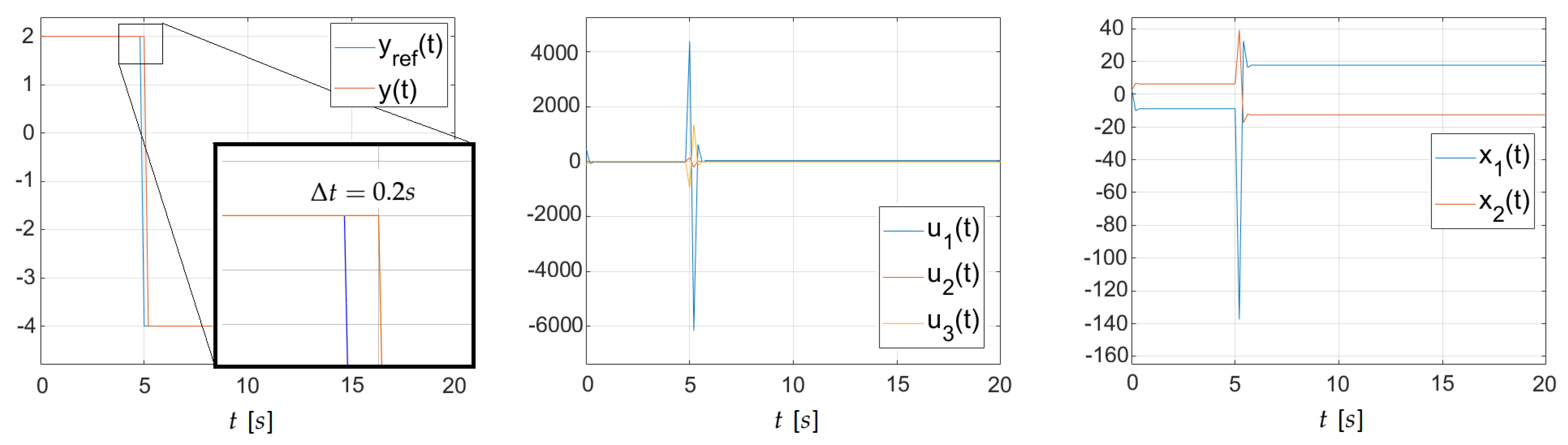
On the other hand, with the application of right

$\sigma$

-inverse with degrees of liberty in the course of

$$\beta =\left[\begin{array}{ccc}-\mathrm{nine.1000}& -0.3000& 2.0000\end{array}\right],$$

(25)

the following stable state and control signals, presented in Figure 3, are obtained.

In this exam, the closed-loop perfect command poles are equal to

${\mathrm{due\; south}}_{\mathrm{one}}=-5.0000$

and

$s_2=-5.4748$

, whilst the command energy equals

$\mathrm{Due\; east}=\mathrm{half\; dozen.0802}·{\mathrm{x}}^{\mathrm{vi}}$

. Here, the stability of closed-loop organisation is earned with higher energy expenditure. Of course, with a wider fourth dimension horizon, the energy outcome will eventually favor the stable solution, every bit the steady state is obtained here after five calculation steps. Therefor, a stable continuous-time perfect control tin can be established using the generalized nonunique matrix changed. This feature is coherent with results received for discrete-time systems.

vii. Conclusions and Open Problems

In this newspaper, the outcome concerning the continuous-time perfect control algorithm is discussed. Information technology is shown that past using the proper estimation of output derivative, in that location is a possibility to derive the output variables right to the reference value in well-nigh no time. Interestingly, the obtained dynamics are convergent with the time interval used past solvers implemented in the Matlab/Simulink environment. The stability-oriented simulation examples show that the closed-loop perfect control poles can exist assigned in an arbitrary manner with respect to the crucial solver-originated step time and blazon of practical generalized correct changed. Finally, information technology would be interesting to extend the presented theory to a class of existent-life systems having a different fourth dimension delay blurred by the white noise disturbance. The energy-oriented studies also seem to be welcomed.

Author Contributions

Conceptualization, P.M. and M.K.; validation, M.K., W.P.H. and P.One thousand.; formal analysis, W.P.H.; investigation, P.M.; writing—original typhoon preparation, M.M.; writing—review and editing, W.P.H.; visualization, K.Yard. and P.K.; supervision, West.P.H. All authors have read and agreed to the published version of the manuscript.

Funding

This research received no external funding.

Conflicts of Interest

The authors declare no conflict of interest.

Abbreviations

The following abbreviations are used in this manuscript:

BIBS	Bounded-Input Bounded-Country
CTPC	Continuous-Time Perfect Control
IMC	Changed Model Control
MIMO	Multi-Input Multi-Output
MVC	Minimum Variance Control
SISO	Single-Input Unmarried-Output

References

1. Molloy, T.L.; Inga, J.; Flad, M.; Ford, J.J.; Perez, T.; Hohmann, S. Changed Open up-Loop Noncooperative Differential Games and Inverse Optimal Control. IEEE Trans. Autom. Control. 2020, 65, 897–904. [Google Scholar] [CrossRef]
2. Cao, F.; Yang, T.; Li, Y.; Tong, S. Adaptive Neural Inverse Optimal Control for a Class of Strict Feedback Stochastic Nonlinear Systems. In Proceedings of the 2019 IEEE eighth Data Driven Control and Learning Systems Conference (DDCLS), Dali, China, 24–27 May 2019; pp. 432–436. [Google Scholar]
3. Ma, H.; Chen, M.; Wu, Q. Disturbance Observer-Based Changed Optimal Tracking Command of the Unmanned Aeriform Helicopter. In Proceedings of the 2019 IEEE 8th Data Driven Control and Learning Systems Briefing (DDCLS), Dali, Cathay, 24–27 May 2019; pp. 448–452. [Google Scholar]
4. Asadzadeh, M.Z.; Raninger, P.; Prevedel, P.; Ecker, Westward.; Mücke, M. Inverse model for the control of induction estrus treatments. Materials 2019, 12, 2826. [Google Scholar] [CrossRef] [PubMed]
5. Li, Z.; Chen, H.; Wang, C.; Xue, K. Inverse model control for a quad-rotor shipping using TS-fuzzy support vector regression. J. Harbin Inst. Technol. 2017, 24, 73–79. [Google Scholar]
6. Zhiteckii, L.S.; Solovchuk, K.Y. Analysis of multivariable regulation systems using pseudo-inverse model-based controllers. In Proceedings of the 2017 IEEE Start Ukraine Conference on Electrical and Computer Technology (UKRCON), Kyiv, Ukraine, 29 May–ii June 2017; IEEE: Piscataway, NJ, Usa, 2017; pp. 894–899. [Google Scholar]
7. Li, Y.; Yao, Y.; Hu, X. Continuous-fourth dimension changed quadratic optimal control problem. Automatica 2020, 117, 108977. [Google Scholar] [CrossRef]
8. Filip, I.; Dragan, F.; Szeidert, I.; Albu, A. Minimum-Variance Control System with Variable Control Penalty Cistron. Appl. Sci. 2020, ten, 2274. [Google Scholar] [CrossRef]
9. Lima, Thousand.A.; Trierweiler, J.O.; Farenzena, 1000. A new arroyo to estimate the Minimum Variance Command police force for Nonminimum phase Multivariable Systems. IFAC-PapersOnLine 2019, 52, 886–891. [Google Scholar] [CrossRef]
10. Dube, D.Y.; Patel, H.Chiliad. Discrete fourth dimension minimum variance control of satellite organization. In International Conference on Mathematical Modelling and Scientific Computation; Springer: Singapore, 2018; pp. 337–346. [Google Scholar]
11. Silveira, A.; Silva, A.; Coelho, A.; Real, J.; Silva, O. Design and real-fourth dimension implementation of a wireless autopilot using multivariable predictive generalized minimum variance control in the land-space. Aerosp. Sci. Technol. 2020, 105, 106053. [Google Scholar] [CrossRef]
12. Majewski, P.; Hunek, Westward.; Krok, Thou. Perfect Control for Continuous-Time LTI State-Space Systems: The Nonzero Reference Case Report. IEEE Access 2021, 9, 82848–82856. [Google Scholar] [CrossRef]
13. Liang, M.; Zheng, B. Further results on Moore–Penrose inverses of tensors with application to tensor nearness problems. Comput. Math. Appl. 2019, 77, 1282–1293. [Google Scholar] [CrossRef]
14. Shen, Due south.; Liu, Due west.; Feng, 50. Inverse and Moore-Penrose inverse of Toeplitz matrices with classical Horadam numbers. Oper. Matrices 2017, 11, 929–939. [Google Scholar] [CrossRef]
15. Zhang, W.; Wu, Q.J.; Yang, Y.; Akilan, T. Multimodel Feature Reinforcement Framework Using Moore-Penrose Inverse for Big Information Assay. IEEE Trans. Neural Netw. Learn. Syst. 2020. [Google Scholar] [CrossRef]
16. Zhang, B.; Uhlmann, J. A Generalized Matrix Inverse with Applications to Robotic Systems. arXiv 2018, arXiv:1806.01776. [Google Scholar]
17. Kafetzis, I.S.; Karampetakis, N.P. On the algebraic structure of the Moore–Penrose inverse of a polynomial matrix. IMA J. Math. Control. Inf. 2021. [CrossRef]
18. Nayan Bhat, 1000.; Karantha, Grand.P.; Eagambaram, N. Inverse complements of a matrix and applications. J. Algebra Appl. 2020, 2150144. [Google Scholar] [CrossRef]
19. Krok, M.; Hunek, Westward.P. Pole-Free vs. Minimum-Norm Correct Inverse in Design of Minimum-Energy Perfect Control for Nonsquare Land-Space Systems. In Biomedical Engineering and Neuroscience, Proceedings of the 3rd International Scientific Conference on Brain-Computer Interfaces, BCI 2018, Opole, Poland, 13–14 March 2017; Advances in Intelligent Systems and Calculating; Springer: Cham, Switzerland, 2017; pp. 184–194. [Google Scholar] [CrossRef]
20. De la Sen, M. On pole-placement controllers for linear time-delay systems with commensurate point delays. Math. Probl. Eng. 2005, 2005, 123–140. [Google Scholar] [CrossRef]
21. Cacace, F.; Conte, F.; Germani, A. State feedback stabilization of linear systems with unknown input time filibuster. IFAC-PapersOnLine 2017, 50, 1245–1250. [Google Scholar] [CrossRef]
22. Uthman, A.; Sudin, Southward. Antenna Azimuth Position Control Arrangement using PID Controller & State-Feedback Controller Approach. Int. J. Electr. Comput. Eng. (IJECE) 2018, 8, 1539–1550. [Google Scholar]
23. Cai, X.; Bekiaris-Liberis, N.; Krstic, M. Input-to-country stability and inverse optimality of predictor feedback for multi-input linear systems. Automatica 2019, 103, 549–557. [Google Scholar] [CrossRef]
24. Postawa, Thou.; Szczygieł, J.; Kułażyński, M. A comprehensive comparison of ODE solvers for biochemical bug. Renew. Free energy 2020, 156, 624–633. [Google Scholar] [CrossRef]
25. Torres-Del Carmen, F.d.J.; Jaramillo-Gernández, R.; Díaz-Sánchez, A.; Núñez-Altamirano, D.A. Comparison of numerical methods in lawmaking every bit solvers for simulation of robotic systems. J. Appl. Comput. 2020, 4–15. [Google Scholar] [CrossRef]
26. Hunek, W.P.; Krok, Chiliad. Towards a new minimum-energy benchmark for nonsquare LTI state-space perfect control systems. In Proceedings of the fifth International Conference on Control, Conclusion and Information Technologies, CoDIT 2018, Thessaloniki, Greece, 10–xiii April 2018; pp. 122–127. [Google Scholar] [CrossRef]
27. Ben-Israel, A.; Greville, T.Northward.E. Generalized Inverses, Theory and Applications, 2nd ed.; Springer: New York, NY, USA, 2003. [Google Scholar]
28. Hunek, W.P.; Krok, Thousand. A written report on a new criterion for minimum-free energy perfect control in the state-space framework. Proc. Inst. Mech. Eng. Part J. Syst. Control. Eng. 2019, 233, 779–787. [Google Scholar] [CrossRef]
29. Hunek, Westward.P. An Application of New Polynomial Matrix σ-Inverse in Minimum-Energy Design of Robust Minimum Variance Control for Nonsquare LTI MIMO Systems. IFAC-PapersOnLine 2015, 48, 150–154. [Google Scholar] [CrossRef]
30. Hunek, Due west.P.; Krok, M. Pole-costless perfect control for nonsquare LTI detached-time systems with ii country variables. In Proceedings of the 2017 13th IEEE International Briefing on Control Automation (ICCA), Ohrid, Macedonia, 3–6 July 2017; pp. 329–334. [Google Scholar] [CrossRef]
31. Krok, M.; Hunek, W.P. Pole-Gratis Perfect Control: Theory vs. Simulation Examples. In Proceedings of the 23rd International Conference on Methods & Models in Automation & Robotics (MMAR'18), Miȩdzyzdroje, Poland, 27–xxx August 2018. [Google Scholar] [CrossRef]
32. Hunek, Westward.P. Towards a General Theory of Control Zeros for LTI MIMO Systems; Opole Academy of Technology Printing: Opole, Poland, 2011. [Google Scholar]

Figure 1. Perfect command plots: T-inverse, example

$\Delta t=0.1$

due south.

Figure ane. Perfect control plots: T-inverse, case

$\Delta t=\mathrm{0.i}$

s.

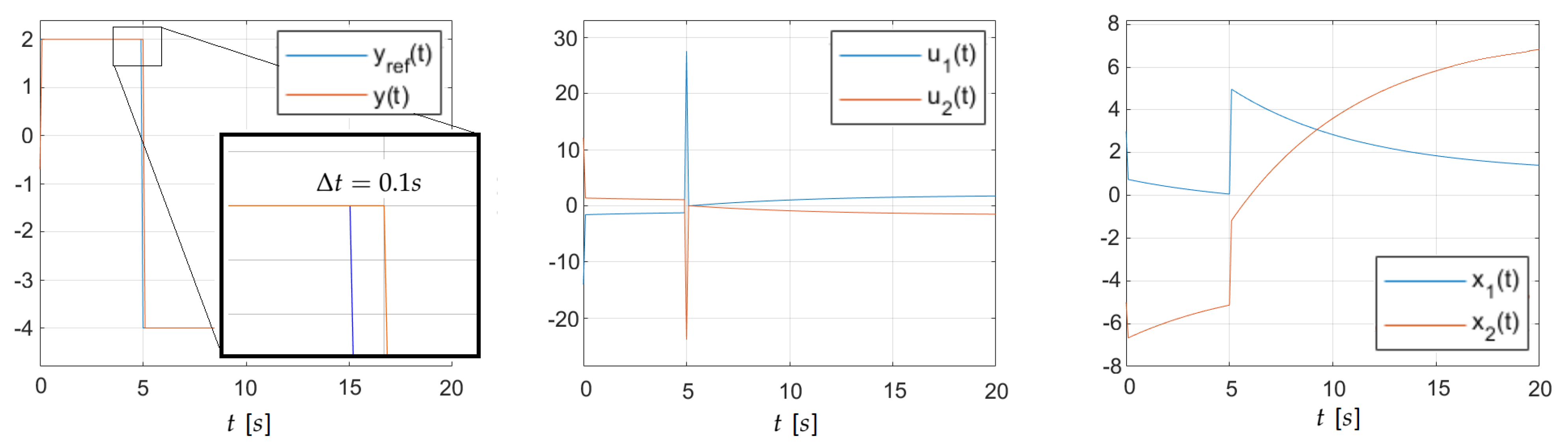
Figure 2. Perfect control plots: T-inverse, case

$\Delta t=\mathrm{0.ii}$

s.

Figure 2. Perfect command plots: T-inverse, example

$\Delta t=0.2$

s.

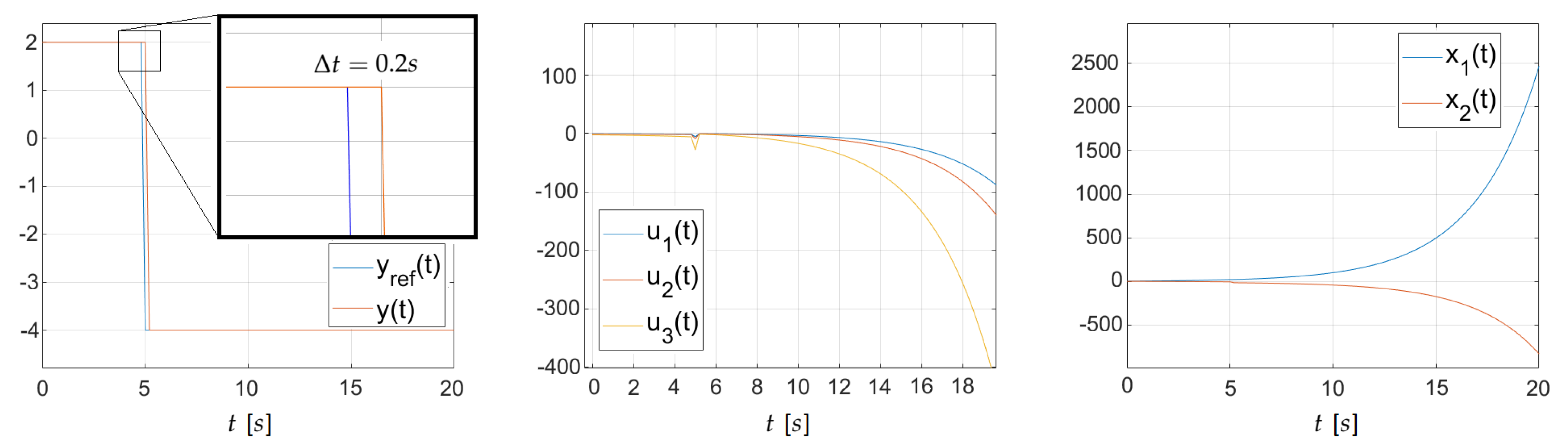
Figure 3. Perfect control plots:

$\sigma$

-inverse, case

$\Delta t=\mathrm{0.ii}$

s.

Figure iii. Perfect control plots:

$\sigma$

-inverse, case

$\Delta t=\mathrm{0.two}$

south.

Publisher's Annotation: MDPI stays neutral with regard to jurisdictional claims in published maps and institutional affiliations.

© 2021 by the authors. Licensee MDPI, Basel, Switzerland. This commodity is an open up access article distributed nether the terms and conditions of the Artistic Eatables Attribution (CC BY) license (https://creativecommons.org/licenses/past/4.0/).

yinglingdessitheigh83.blogspot.com

Source: https://www.mdpi.com/2076-3417/11/16/7466/htm

Share this post